6-2

Visual Instruction of Stress Smoothing

Understanding stress recovery and smoothing

This educational function is intended to help explaining or understanding the concepts and the procedures of the stress recovery and smoothing. Using this function, you can also visualize various computational aspects of the procedures and make comparison between methods.

Simulating the process of conjugate recovery and smoothing

The process of strain recovery and smoothing can be simulated by a series of operations. Recovery and smoothing by the conjugate method proceeds by the following steps:

	Compute the strains at integration points within an element.
	Extrapolate them to the nodes of the element.
	Repeat step 2) for all elements.
	Compute the smoothed strains at a node by averaging the strains obtained from each of the element meeting at the node.
	Repeat step 4) for all nodes.
	Compute the strain at a point within an element by interpolating the nodal values of the element.

Each phase of the above procedure can be simulated by the following steps:

	1) Set the method of computation as “Conjugate.”
		Choose “Conjugate” item from “Method 1” submenu of menu, and choose “Method 1” item from “Displayed Method” submenu.
	2) Set the view direction of image on “Recovery and Smoothing” window.
		The view direction should be set in oblique angle so that the level surface representing the strain distribution can be 3-dimensionally visualized.
	3) Set rendering mode to ”By Wireframe” or “By Shading” by choosing the corresponding menu item from menu.
		The strain distribution is represented by level surfaces under these rendering modes.
	4) Select an element to display the strain computation.
		Click the element on the main window. Only the strain of the selected element is displayed on “Recovery and Smoothing” window.
	5) Display the magnitude of strain at each integration point of the element.
		Choose “Show I.P. Legs” item from menu. The height of a leg represents the magnitude of the strain recovered at that point. If the legs are covered by the level surface, hide the level surface by choosing the menu item, “Hide Level Surface.”
	6) Visualize the extrapolation of the strains at integration points
		The level surface re p resents the surface extrapolating the strains from the integration points to every point over the element. If “Hide Level Surface” item in menu is checked, the surface is not shown. In this case, choose the menu item again. Then, the item is unchecked, and the surface appears.
	7) Display the extrapolated values of strains at nodal points.
		Choose "Show Node Legs"" menu item to display the node legs. The height of a leg represents the magnitude of the strain extrapolated to the corresponding node.
	8) Visualize strain field over the entire model.
		Select all the elements on the main menu. Then, the level surfaces and node legs in the entire region are displayed. This visualizes the overall distribution of strain and shows discontinuity of strain across element boundaries.
	9) Visualize the smoothed strain field over the entire model .
		Change the method of computation to "Conjugate with Smoothing" by selecting the menu item. The strain at a node is computed by averaging the values of all the elements connected at the node. This strain field has smooth and continuous variation.

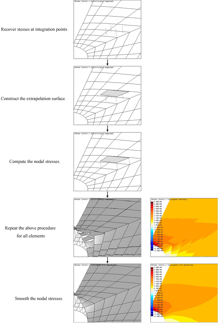
< Simulation of conjugate recovery and smoothing process >

Simulating the process of nodal recovery and smoothing

According to nodal recovery, the strain at a node is directly computed from the strain-displacement relationship at the node. This method is seldom used in actual finite element software, but provided for the educational purpose of comparing the method with conjugate stress smoothing. This method goes through a process similar to but simpler than that of conjugate recovery and smoothing.

	Compute the nodal strains for each of the elements.
	Compute the smoothed strains at a node by averaging the strains obtained
	Compute the smoothed strains at a node by averaging the strains obtained from each of the element meeting at the node.
	Repeat the foregoing step for all nodes.
	Compute the strain at a point within an element by interpolating the nodal values of the element.

Each phase of the above procedure can be simulated by the following steps:

	1) Set the method of computation as “Nodal Recovery”.
		Choose “Nodal Recovery” item from “Method 1” submenu of menu, and choose “Method 1” item from “Displayed Method” submenu.
	2) Set the view direction of image on “Recovery and Smoothing” window.
		The view direction should be set in oblique angle so that the level surface representing the strain distribution can be 3-dimensionally visualized.
	3) Set rendering mode to “By Wireframe” or “By Shading” by choosing the corresponding menu item from menu.
		The strain distribution is represented by level surfaces under these rendering modes.
	4) Select an element to display the strain computation.
		Click the element on the main window. Only the strain of the selected element is displayed on “Recovery and Smoothing” window.
	5) Display the strains computed at nodal points.
		Choose “Show Node Legs” menu item to display the node legs. The height of a leg represents the magnitude of the strain computed at the node.
	6) Visualize strain field over the entire model.
		Select all the elements on the main menu. Then, the level surfaces and node legs in the entire region are displayed. This visualizes the overall distribution of strain and shows discontinuity of strain across element boundaries.
	7) Visualize the smoothed strain field over the entire model.
		Change the method of computation to “Nodal Recovery with Smoothing” by selecting the menu item. The strain at a node is computed by averaging the values of all the elements connected at the node. This strain field has smooth and continuous variation.

Examining the intermediate results of computation

The process of computing strains and stresses can be displayed in text form on “Recovery and Smoothing” window, which includes all the data obtained from intermediate computations. They are arranged in hierarchical tree view in accordance with the computational procedure. A data item is expanded or collapsed by clicking or mark which is in front of its title. The contents of the display vary depending on the method of recovery and smoothing as summarized in the following.

“Computed Pointwise” : Strains are recovered directly at the point specified by mouse click. The following items are computed only at this point.
	- Node data
		Coordinates, displacements
	- Property
		Elastic modulus and poisson? ratio, stress-strain matrix
	- Shape function and Jacobian matrix at the clicked point
		Natural coordinates, cartesian coordinates, shape function derivative in natural coordinates, shape function derivatives in Cartesian coordinates, Jacobian matrix, Jacobian inverse
	- Strain and displacement matrix at the clicked point
	- Strains and stresses at the clicked point
		Natural coordinates, shape functions, strains, stresses

	“Conjugate” : Strains are recovered at every integration point. They are extrapolated to nodes using extrapolation matrix. The strains and stresses at the clicked point are obtained by interpolating from the nodal values.
		- Node data
		- Property
		- Shape function and Jacobian matrix at each integration point
		- Strain and displacement matrix at each integration point
		- Strains at each integration point
		- Extrapolation matrix
		- Strains at each node
		- Strains and stresses at the clicked point

	“Conjugate with Smoothing” : The nodal strain field obtained by the above “Conjugate” method are smoothed. Thus, this method has one more step than the above method.
		- Node data
		- Property
		- Shape function and Jacobian matrix at each integration point
		- Strain and displacement matrix at each integration point
		- Strains at each integration point
		- Extrapolation matrix
		- Strains at each node
		- Smoothed strains at each node
		- Strains and stresses at the clicked point

	“Nodal Recovery” : Strains are computed directly at every node based on the strain-nodal displacement relationship at the node. Therefore, extrapolation stage is not necessary for this method.
		- Node data
		- Property
		- Shape function and Jacobian matrix at each node
		- Strain and displacement matrix at each node
		- Strains at each node
		- Strains and stresses at the clicked point

	“Nodal Recovery with Smoothing” : The nodal strain field obtained by the above "Nodal Recovery" method is smoothed by this method. Thus, this method has one more step than the above method. The strains at the specified point are obtained by interpolating from the smoothed strains.
		- Node data
		- Property
		- Shape function and Jacobian matrix at each node
		- Strain and displacement matrix at each node
		- Strains at each node
		- Smoothed strains at each node
		- Strains and stresses at the clicked point

Comparing two different methods

The characteristics of a method can be understood more clearly by comparing the computed strains or stresses with those obtained by other methods. The difference of the strain fields from two diff e rent methods can be visualized by choosing “Method 1 - Method 2” item from “Displayed Method” submenu of menu. For example, the difference of the strain energy density field computed by “Conjugate” and the one by “Conjugate with Smoothing” can be obtained in the following procedure.

	1) Select “Energy Density” for strain component.
		Choose “Energy Density” item from “Strain Component” submenu of menu.
	2) Set the method of computation as “Conjugate”.
		Choose “Conugate” item from “Method 1” submenu.
	3) Set the comparing method of computation as “Conjugate with Smoothing.”
		Choose “Conugate with Smoothing” item from “Method 2” submenu.
	4) Set the displayed method as “Method 1 - Method 2”.
		Choose “Method 1- Method 2” item from “Displayed Method” submenu.

The image in the following figure shows the difference of the strain energy density fields obtained from the two methods.

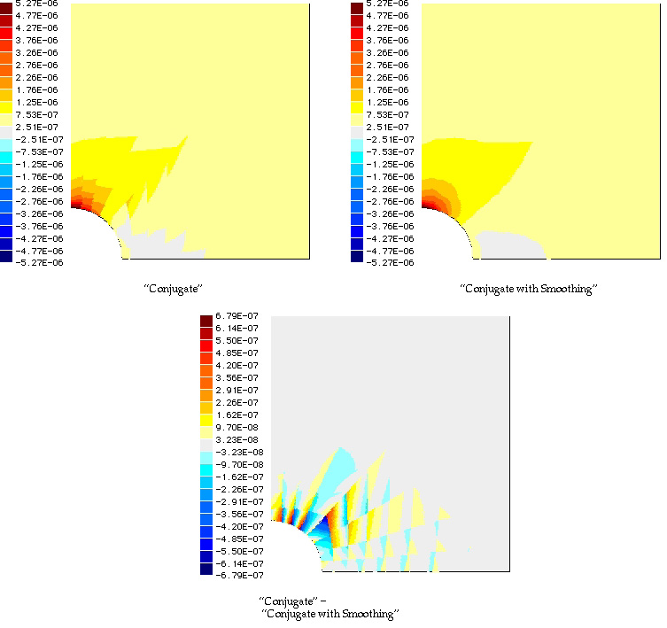
< Graphical comparison of 2 different methods >