Visual Instruction of Stress Smoothing
|
Visual Instruction of Stress Smoothing |
|
|
| |
||
Basic usage of the function
The stress recovery and smoothing can be visualized only for a model which
is solved. There f o re, a model should be created and solved before starting
thisfunction. The basic usage of the function is described below.
Starting the function
This instructional function is initiated by choosing “Display Stress Recovery”
item from “FEM Simulation” submenu of ![]() menu. The following few steps should be taken in order to start displaying the
element stiffness information.
menu. The following few steps should be taken in order to start displaying the
element stiffness information.
|
1) Create a model, and assign element properties and boundary conditions |
||
|
Create a model by mesh generation and assign the data necessary for solving the model. |
||
|
2) Solve the model by choosing "Solve" item from |
||
|
The model should be solved, and thus the nodal displacements should be obtained for computation of the strains. |
||
|
3) Select “Display Stress Recovery” item from “FEM Simulation” submenu
of |
||
|
Then, “Recovery and Smoothing” window appears on the screen. The window
is initially blank until one or more elements are selected from the mesh
on the main window. |
||
|
4) Select the elements from the mesh on the main window. |
||
|
The selected elements are displayed on "Recovery and Smoothing" window. |
||
|
5) Choose the strain component to display. |
||
|
The strain image is not displayed until the strain component is chosen
from “Stress Component” submenu of |
||
Ending the function
The function is terminated by closing “Recovery and Smoothing” window. Clicking the close box of the window will close the window. The function may also be terminated by starting other menu function.
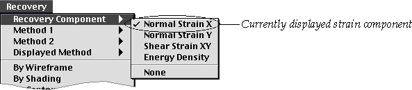
Selecting the strain component to display
The displayed strain component can be changed by choosing new item from “Stress Component” submenu. The menu item with a check mark in front indicates the currently displayed strain component. In order to remove the strain image, choose “None” item. View transformation on “Recovery and Smoothing” window can be made faster by removing the strain image temporarily.
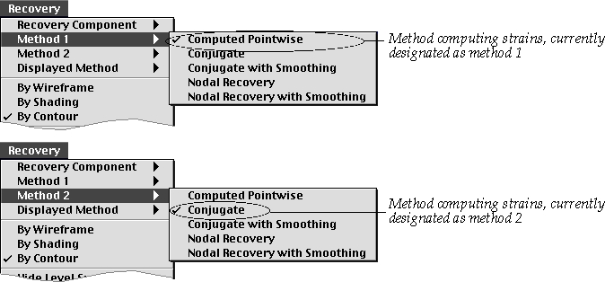
Designating methods of strain computation
The strain image on “Recovery and Smoothing” window represents the value of the strain component computed at every pixel. This software provides 5 different methods of computing strains as follows:
|
“Computed Pointwise” : The strain is computed using the strain-nodal displacement relationship at every pixel. Neither extrapolation nor interpolation of strain is applied. |
|
|
“Conjugate” : The nodal strains are extrapolated from the strains at integration points by conjugate method, and the strain at a pixel is obtained by interpolating from the nodal values. |
|
|
“Conjugate with Averaging” : The nodal strains in each element are obtained by the above method. The final value of a node is evaluated by averaging the different nodal values of the elements connected to the node. |
|
|
“Nodal Recovery” : The nodal strains are computed directly from the strainnodal displacement relationship at the node. |
|
| ‘’Nodal Recovery with Averaging” : The nodal strains are first computed by nodal recovery, and then evaluated by averaging the different nodal values of the elements connected to the node. The strain image can be obtained by applying any one of the above methods, or offsetting two different methods. To make it easy to set and identify the method of computing strain, two methods out of the above 5 can be designated as method 1 and method 2 respectively. To designate method 1 and method 2, choose one item from each of “Method 1” and “Method 2” submenus. |
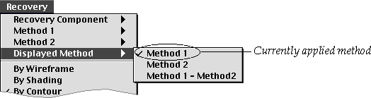
Selecting the method of obtaining strain image
The strain image can re p resent the strain computed by one of method 1 and method 2, or the value obtained by offsetting the strains computed by the two methods. The method of obtaining the strain image can be selected from the menu items of “Display Method” submenu.
|
“Method 1”: Strain image represents the value computed by method 1. |
|
|
“Method 2”: Strain image represents the value computed by method 2. |
|
|
“Method 1 - Method 2”: The strain image re p resents the value obtained by offsetting the strain computed by method 2 from the strain computed by method 1. |
The menu item corresponding to the currently applied method is checked in front. The contents of “Recovery Text” window are also determined by this menu selection. However, if “Method 1 - Method 2” is selected, “Method 1” is applied for “Recovery Text” window.
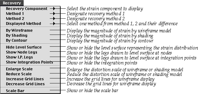
Selecting the rendering method
There are 3 diff e rent modes of re p resenting the strain distribution: wire
frame, shading and contouring. The mode can be set by choosing the corresponding
item from ![]() menu.
menu.
|
“By Wireframe”: Choose this item to re p resent the strain distribution by a level surface rendered in wireframe. The grid lines of the wireframe are drawn with hidden line removal. |
|
|
“By Shading”: Choose this item to represent the strain distribution by a level surface with smooth shading. |
|
|
“By Contour”: Choose this item to represent the strain distribution by contours. |
There appears check mark in front of the menu item set for the rendering mode.
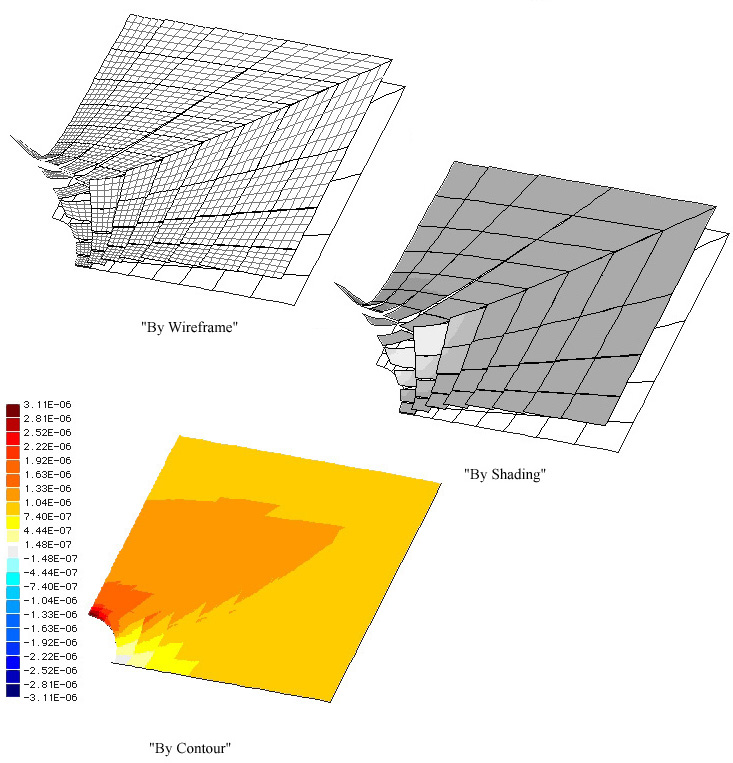
< Methods of rendering strain >
Showing or hiding the level surface of strain distribution
If the rendering method is set as “By Wireframe” or “By Shading”, the strain
distribution is represented by a level surface. Choosing “Hide Level Surface”
item from ![]() menu will make the level surface invisible. The height of the level surface
at integration points can be revealed more clearly by hiding the leve surface
itself. Choosing the item again will make the level surface visible.
menu will make the level surface invisible. The height of the level surface
at integration points can be revealed more clearly by hiding the leve surface
itself. Choosing the item again will make the level surface visible.
Showing or hiding the node legs
code leg is a line drawn at a node from the base plane to the level surface. Choose “Show Node Legs” items in order to show or hide node legs. The menu item is checked when node legs are shown.
This function is valid only when the rendering method is set as “By Wireframe” or “By Shading.” “By Wireframe” “By Shading” “By Contour”
Showing or hiding the I.P. legs
I . P. leg is a line drawn at an integration point from the base plane to the level surface. Choose “Show I.P. Legs” items in order to show or hide I.P. legs. The menu item is checked when I.P. legs are shown. This function is valid only when the rendering method is set as “By Wireframe” or “By Shading.”
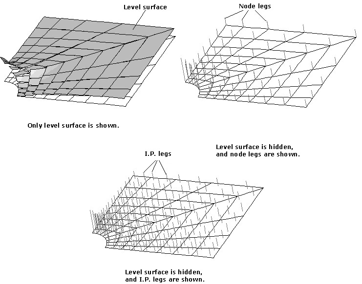
< Showing and hiding level surface, node legs or I.P. legs >
Enlarging or reducing the scale of the level surface
The scale of the level surface is the height of the surface representing the
unit value of strain. Choose “Enlarge Scale” item from ![]() menu in order to enlarge the scale of the level surface. Choose “Reduce
Scale” item in order to reduce the scale of the level surface. These functions
are valid only when the rendering method is set as “By Wireframe” or “By Shading.”
menu in order to enlarge the scale of the level surface. Choose “Reduce
Scale” item in order to reduce the scale of the level surface. These functions
are valid only when the rendering method is set as “By Wireframe” or “By Shading.”
Increasing or decreasing the number of grid lines
Level surface consists of grids which are used for rendering the surface by
wireframe or shading. The number of grid lines can be increased or decreased
by choosing “Increase Grid Lines” or “Decrease Grid Lines” item from ![]() menu.
menu.
This function is valid only when the rendering method is set as “By Wireframe”
or “By Shading.”
Showing or hiding the scale bar
The scale bar is drawn to the left of the contour image of the strain distribution,
and can be made visible or invisible by choosing “Scale Bar” item of ![]() menu. This function is valid only when the rendering method is set as “By Contour.”
menu. This function is valid only when the rendering method is set as “By Contour.”
Highlighting element
The boundary lines of an element are popped up on recovery and SmoothingO window,
as you place the screen cursor over the element. As you move the cursor, this
element highlighting transfers from one element to another. If you move the
cursor out of the window, the element highlighting disappears, and no element
is marked.
Getting details of the strain computation
The information on the strain computation can be displayed in text form. Click
an element on “Recovery and Smoothing” window. Then, “Recovery Text” window
opens, and the details of the computation for the element are displayed on the
window. The information is arranged in hierarchical tree view. At the beginning,
only the root level items are shown. An item is expanded or collapsed by clicking
![]() or
or
![]() mark which is in front of the title of each item.
mark which is in front of the title of each item.
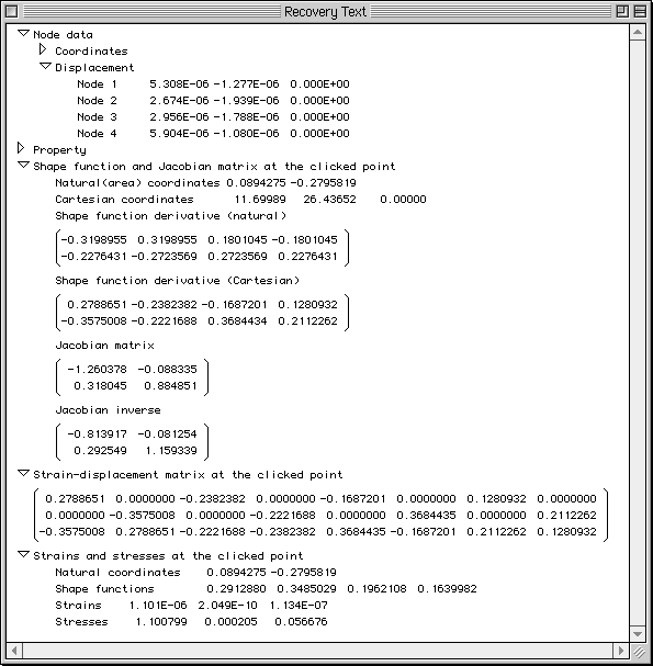
< An example of partially expanded information tree of strain computation >
|
|
|
|