Examining Eigenvalues and Eigenvectors of Stiffness

Examining finite element characteristics by eigen modes

The characteristics and the validity of an element or an assembly of elements can be measured by examining the eigenvalues and the eigenvectors of their stiffness matrix. The eigenvalues are related to strain energy, and thus can be used to detect the rigid body modes and the spurious zero energy modes of the system. Their eigenvectors are interpreted as displacement modes, and thus give insight on the behavior of the system. The strains may be constructed from the gradients of the eigenvectors, and will give further insight into the computational aspects of a finite element. The quality of an element can also be evaluated by the eigenvalues.

Identifying the rigid body modes

A rigid body mode is a displacement mode without deformation and incurs no strain energ y. Accordingly, the eigenvalue associated with a rigid body mode should bear zero value. However, all zero eigenvalues do not necessarily represent rigid body modes. There is a kind of zero eigenvalue called a spurious mode. Rigid body modes can be distinguished from spurious zero energy modes by the appearance of their graphically rendered eigenvectors. Animation of the modes may give clearer distinction.

It is a necessary condition for correct convergence of the finite element solution that the elements used in the model should be able to re p resent the rigid body modes properly. The required number of rigid body modes of an element varies depending on the analysis types as shown below.

The required number of rigid body modes listed above for each type of analysis applies not only for a single element but also for an assembly of elements without boundary constraints. If boundary constraints are applied to the eigenvalue model, the total number of eigenvalues is reduced by the number of constrained DOF. At the same time, the number of zero eigenvalues is also reduced by the number of constrained rigid body modes. One can easily identify whether an element or an assembly of elements has proper rigid body modes, by examining the eigenvalues and associated eigenvectors.

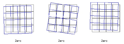
< Rigid body modes of a plane stress example >

Detecting spurious zero energy modes

There is another kind of zero eigenvalue re p resenting displacements which undergo deformation but computationally yield zero strain energy. These zero eigenvalues are called spurious zero energy modes. As shown in the figure below, the eigenvectors of the spurious modes distort the element shapes, although the corresponding eigenvalues are zero. If the number of zero eigenvalues is greater than the number of the required rigid body modes, spurious modes are always involved in the model. The existence of spurious modes within the model is a critical factor for its validity. The spurious modes may be detected not only in a single element but also in an assembly of elements.

If the number of zero eigenvalues is greater than the number of the required rigid body modes, spurious modes are always involved in the model. The existence of spurious modes within the model is a critical factor for its validity. The spurious modes may be detected not only in a single element but also in an assembly of elements.

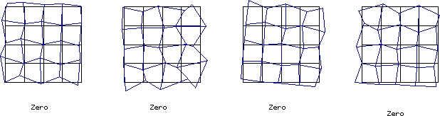
< Spurious zero energy modes of a palne stress example >

Probing the computational pitfall of spurious modes

Spurious zero energy mode re p resents the state of deformation which causes no strain energy. Deformation without strain or strain energy is possible only in computation. Such a computational pitfall arises when the strains due to the deformation happen to be zero at all the integration points. Under such acircumstance, the strain energy is perverted computationally to be zero because the stiffness matrix is evaluated from the strain-displacement relationships at the integration points.

The computational aspect of spurious modes can be probed by displaying their eigen mode equivalents of strain. Choose the strain component using “By Contour” submenu in menu. Then, the strain field is expressed by contours in “Eigen Modes” window. As shown below for an 8-node element, all the strain components are zero at every integration point, although the element is not strain-free. With a rigid body mode, each strain component is uniformly zero over the element.

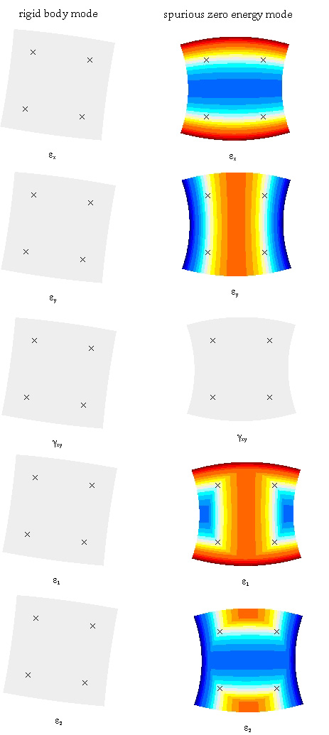
< Comparison of strains under rigid body mode and spurious zero energy mode >

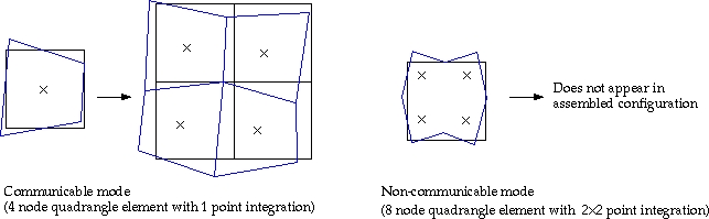
Comparing communicable and non-communicable modes

Some spurious zero energy modes appearing at an element may or may not disappear in an assembly of elements. If it disappears, it is called a noncommunicable mode. Otherwise, it is called communicable mode. Noncommunicable modes are less problematic in finite element computations than communicable modes.

In the example shown below, two plane stress models are compared. One consists of 4 node quadrilateral elements with 1 point integration, and the other consists of 8 node quadrilaterals with 2 X 2 integration. The 4 node quadrilateral elements show so-called “Hour-glass mode” which is a communicable mode. And thus, the spurious mode still appears for assembly of the elements as well. On the other hand, the spurious mode in the 8 node element is non-communicable . And the mode disappears in assembled configuration. This eigen mode shape indicates that two adjacent elements cannot have the mode at the same time. As a result, the assembly of 2 or more elements will not possess this spurious mode. Spurious zero energy modes may disappear after the model is constrained properly by boundary conditions. But communicable modes may persist even after boundary conditions are applied.

< Comparison of strains under rigid body mode and spurious zero energy mode >

Observing the effect of integration order on eigen modes

Spurious zero energy modes represent the rank deficiency of the stiffness matrix, which is attributable in many cases to insufficient order of numerical integration. In uch cases, spurious modes can be eliminated by increasing the order of integration. The effect of integration order can be observed by examining how the eigen modes hange when the integration order is increased or decreased. Use “Increase Integration” or “Reduce Integration” item in menu to change the integration rule. And inspect especially the zero eigenvalues and their eigenvectors. The number of zero eigenvalues tends to increase, and accordingly include spurious modes, as the integration order is reduced. The eigen modes in an 8 node quadrilateral element are exemplified in the figure below. The example shows that 4 zero eigenvalues are brought by 2 X 2 integration. As described earlier in this section, 3 rigid body modes are expected in a plane stress case. However, only 1 zero eigen mode appears to be a rigid body mode, but not the other 3 modes. In fact, the rigid body modes are mixed with the spurious mode in this display. However, we may construe that there are 3 rigid body modes and 1 spurious mode in this case. On the other hand, the spurious mode disappears in case of 3 X 3 integration. There are 3 zero eigenvalues, and all of their eigen modes can be easily identified as rigid body modes. Reduction of the integration order to 1 X 1, if available, will increase the number of spurious modes to 10.

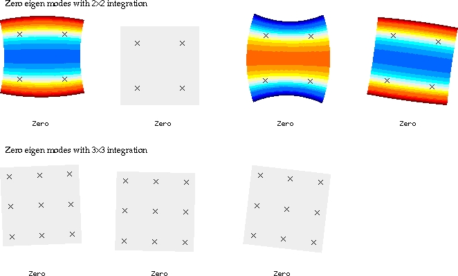
< Examining the effect of integration order on the zero eigen modes >

Testing the geometric isotropy

Geometric isotropy is a property of an element related to the convergence of the finite element solution. This property is not essential, but desirable for correct convergence. If an element does not have any pre f e r red directions, it is called geometrically isotropic, or geometrically invariant. This property can be tested by using the eigenvalues of the stiffness matrix of an element or assembled elements. If a model is geometrically isotropic, the eigenvalues of its stiffness matrix should be invariant regardless of its coordinate transformation. In order to preform such a test efficiently, it is desirable to create two models with identical shape and properties, but with different directions. This can be achieved easily by the following steps:

	1) Create a model.
		Generate mesh of a finite element model for which the eigen modes are to be examined.
	2) Activate “Duplicate and Revolve” function.
		Choose “Revolve item from “Duplicate and “ submenu of menu . Then, “Dup & Revolve” dialog appears on the screen.
	3) Set the angle of rotation in the dialog.
		Insert the text of the angle in the editable text box in the dialog.
	4) Select the model and press key.
		is initially disabled, but becomes enabled when the model is selected. Pressing the key will set the model as the object for duplication. The button turns into .
	5) Input the axis of revolution and press .
		The axis of revolution should be vertical to XY plane in a plane stress case. Thus, it is more convenient way of inputting the axis to type the coordinates of the two end points in the editable text boxes at the bottom of the tool palette. button is initially disabled, but becomes enabled when the axis input is complete. Press the button. Then, the model is duplicated with rotation by the specified angle.

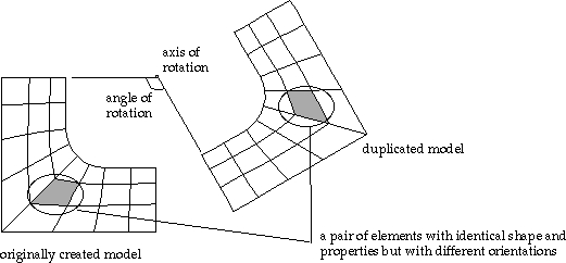
< A pair of models with different orientations for geometric isotropy test >

Geometric isotropy may be inspected either at element level, or for the entire model. The geometric isotropy of an element can be examined with a pair of elements with equal shape and properties but with diff e rent orientations. If the pair of elements has the same eigenvalues, the element is geometrically isotropic. As an example, a pair of elements (shaded in the above figure) are sampled from each of the models, and their eigenvalues are compared. The following list shows that the eigenvalues of one element match exactly with the corresponding values of the other element.

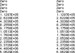
< Comparison of eigenvalues in a pair of elements >

Evaluating the quality of an element

The eigenvalues can be used as a guide measuring the quality of finite elements. The condition number (N) is the ratio of the largest eigenvalue to the smallest. The element with smaller condition number is likely to have better quality or performance. As an example, three 8 node quadrilateral elements are compared with their condition numbers. They are all plane strain elements. One is a square, another is a rectangle, and another is a skewed parallelogram. The condition number of the

square element is the smallest, and that of the parallelogram is the largest. This agrees well with the expectation that the square element has the best quality and the parallelogram has the worst.

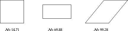
< Comparison of condition numbers >