Examining Eigenvalues and Eigenvectors of Stiffness

Basic usage of the function

The usage of this function described below .

Starting the function

The following few steps are necessary to start displaying eigenvalues and eigenvectors of the stiffness matrix.

Ending the function

The function is terminated by closing “Eigen Modes” window. Clicking the close box of the window will close the window. The function may also be terminated by starting other menu function. menu also disappears from the menu bar as the function terminates.

Forming the stiffness matrix for eigen mode display

The eigenvalues and eigenvectors are computed either for an element stiffness matrix or for an assembled stiffness matrix of multiple elements, depending on the selection of objects prior to starting the function. If one element is selected, eigen modes are computed from the element stiffness matrix of that element. If more than one elements are selected, the stiffness matrix assembled for those elements a re used in the computation. If no element is selected prior to launching the function, the following message appears on the screen.

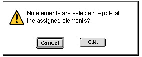
If you click button, all the elements assigned with element properties are assembled in the stiffness matrix for eigen mode display. There are as many eigen modes as the number of d.o.f. included in the stiffness smatrix. All the d.o.f. constrained by boundary conditions are removed from the eigen mode display as well as from the stiffness matrix.

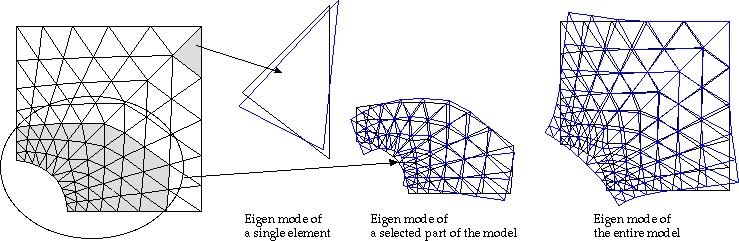
< Various formation of eigen model >

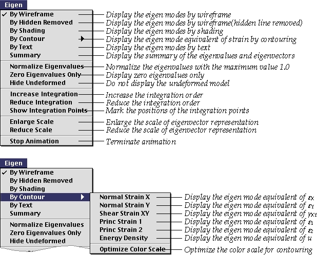
Selecting the form of eigen mode representation

The eigen modes may be represented in various forms including text display. The method of displaying the eigen mode can be set by selecting the corresponding item of menu.

The currently applied form of display is indicated by a checkmark in front of the corresponding menu item.

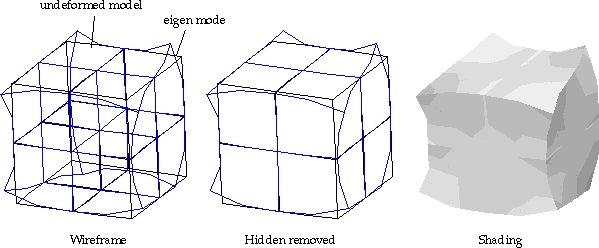
< Types of rendering eigen modes >

Displaying the eigen mode equivalent of strain by contours

As eigenvectors represent displacement modes, their gradients can be interpreted as equivalents of strains. Eigen mode equivalents of strain components are computed on the basis of the strain-displacement relationship to eigenvectors.

They are displayed by contours. Contours of red colors represent positive values, and those of blue colors represent negative values. Near zero values are represented by a white contour. There are a few menu items in “By contour”

submenu to select the strain component and the mode of display.

	“Normal Strain X” : The eigen mode equivalent of normal strain in X direction, eX is displayed by contours.
	“Normal Strain Y” : The eigen mode equivalent of normal strain in Y direction, eY is displayed by contours.
	“Shear Strain XY” : The eigen mode equivalent of shear strain, gX Y i s displayed by contours.
	“Princ Strain 1” : The eigen mode equivalent of maximum principal strain, e1 is displayed by contours.
	“Princ Strain 2” : The eigen mode equivalent of minimum principal strain, e2 is displayed by contours.
	“Energy Density” : The eigen mode equivalent of energy density, U0 i s displayed by contours.
	“Optimize Color Scale” : The color scales are optimized for each eigen mode equivalent of strain so that they are displayed using as many contour lines as possible. If this option is applied, the menu item is check-marked. If not, the contours are scaled uniformly for all eigen mode equivalents of a strain component.

In current version of VisualFEA/CBT, the contouring of eigen mode is available only for plane stress or strain analysis. This contour display is useful in understanding the characteristics of eigen modes.

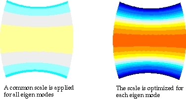
< Contouring eX with different color scales >

Displaying the eigen modes in text

As described above, the numerical values of eigenvalues and eigenvectors can be displayed by text instead of graphics. Select “By Text” item from menu. Then, the contents of "Eigen Modes" window turns into text strings. Initially, only the eigenvalues are displayed. There is a or mark in front of each eigenvalue. This mark alternates between and , whenever it is clicked. Every eigenvalue with mark is expanded with its eigenvectors at the bottom of it. The eigenvectors are hidden for the ones with mark.

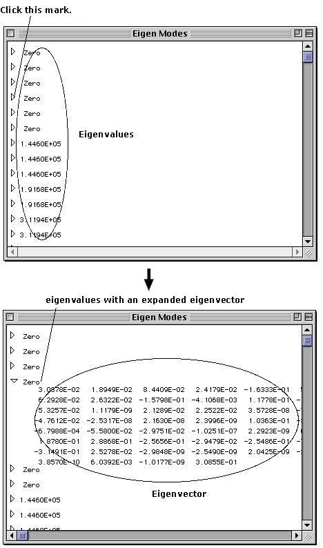
< Displaying eigen modes in text >

Displaying the summary of eigen modes

“Summary” item in menu is to obtain the summarized statistics of the eigen mode analysis. The following items appear on the window.

Animating eigen mode

The eigen modes can be visualized dynamically using animation. Animation works for all types of rendering except text display. If the eigen modes are currently displayed in text, this should be replaced by any other type of rendering before activating animation. For contour display, the contour bands as well as the mode shapes are animated.

Click one of the displayed eigen modes to visualize the mode by animation. Only one mode can be animated at a time. The mode in animation can be switched simply clicking another mode.

Stopping animation

Animation of an eigen mode is stopped by selecting “Stop Animation” item from menu. This menu item is enabled only when animation is going on.

Normalizing eigenvalues

“Normalize eigenvalues” item is used to normalize all the eigenvalues by the maximum value. The maximum value becomes unity after normalization. The other eigenvalues has the value relative to the maximum value. The eigenvalues may be restored to actual value by selecting the item again. The menu item is checked if normalization is applied. Otherwise, it is unchecked.

Displaying zero eigenvalues only

Zero eigenvalues have especially important meaning in eigen mode analysis. They are directly related to the validity of the element, as described in more detail in the later part of this section. In some cases, zero eigenvalues and their associated eigenvectors may be the only information necessary for examination.

Selecting “Zero Modes Only” item from menu toggles the state under which only the zero eigenvalues and their eigenvectors are displayed, and other eigenvalues are hidden.

Showing and hiding the undeformed view of the model

The deformed view of the eigen modes are overlaid over the image of the undeformed shape to make the view more measurable. However, it is sometimes difficult to distinguish the deformed and undeformed views from the overlaid image. In such cases, it is better to display the deformed view only by hiding the undeformed view. The undeformed view of the model can be shown or hidden by choosing “Hide Undeformed” item from menu.

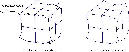
< Showing and hiding the undeformed view >

Increasing or decreasing integration order

The stiffness matrix of an element is computed through numerical integration. The integration rule strongly affects the eigen values and eigenvectors of the stiffness matrix. The order of integration can be increased simply by choosing

“Increase Integration” item from menu. The integration rule is increased to higher order for all types of elements if it is available.

The order of integration can be decreased by choosing “Decrease Integration” item from menu. The integration rule is decreased to lower order for all types of elements if it is available.

There is another method of increasing the integration order. The integration rule may be adjusted for each type of element independently using “Integration Scheme” dialog. The dialog is opened by selecting “Integration scheme” item from menu. It is not necessary to quit “Display Eigen Modes” function to activate “Integration Scheme” dialog. The display of the eigen modes is updated immediately after the integration rule is altered.

Displaying the integration points

It is sometimes necessary to indicate the positions of integration points. In order to display the integration points, select “Show Integration Point” item from menu. They can be hidden by selecting the item again.

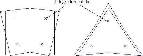
< Showing the integration points >

Enlarging or reducing the scale of deformation

The eigenvectors are visualized by the deformed shape of the model on the basis of the analogy between the eigenvectors and the displacements. Actual eigenvectors may be too small or too large for graphical visualization. So, they are represented as deformations exaggerated with appropriate scale. The optimal scale is automatically determined by the software. This scale can be adjusted if necessary.

The scale is enlarged by selecting “Enlarge Scale” item from menu, and reduced by “Reduce Scale" item. The enlargement or reduction can be made only between the upper and the lower limit of the scale. If the scale reaches the limit, the corresponding menu item is dimmed.

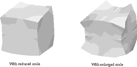
< Enlarging and reducing the scale of the eigenvector display >

Transforming the view of eigen mode

Each of the eigen modes is initially displayed with the same view transformation as that of the model in the main window. This view may be rotated or zoomed for better visualization. These view transformations can be achieved in the same way as transformation of the finite element mesh on the main window. However, the view transformation affects only “Eigen Modes” window, but not main window, while ”Eigen Modes” window is opened. This view transformation is not applicable when the eigen modes are displayed in text.

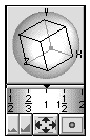	Rotation: Rotate the virtual track ball on the tool palette as shown left.
	Zooming in/out: Adjust the zoom dial or click the zoom button .
	For more detailed description on the use of the tool palette, refer to “View Control” section in Chapter 2.

Panning the whole contents on the window

Use option drag to pan the entire image on “Eigen Modes” window. In other words, press option key and click a point in the window. Then, the cursor turns into . Drag the mouse with button pressed. Then, the entire image on the window moves following the cursor. The movement ends and the shape of the cursor returns to ,when the mouse button is released.

Scrolling, resizing and zooming the window

The contents of “Eigen Modes” window can be scrolled using horizontal or vertical scroll bars. The scroll is applied to text and graphic rendering independently.The window may be resized or zoomed if necessary, by dragging the resize box or clicking the zoom box of the window.