Visual Instruction of Shape Function and Interpolation
|
Visual Instruction of Shape Function and Interpolation |
|
|
| |
||
Basic usage of the function
Described in this section is the basic usage of the function which includes forming and displaying the interpolation model, and also view transformation and rendering options for better visualization.
Starting the function
The following few steps are necessary to start displaying shape functions and their derivatives.
|
1) Create elements with shape function to be examined. Generate mesh with elements of the shape and the order for which the desired shape function is employed. |
|
|
2) Assign element properties. Only elements assigned with element properties are valid for displaying their shape functions. |
|
|
3) Select “Shape Function” item from “Stiffness” submenu of “Shape Function” window appears on the screen, and |
Ending the function
The function is terminated by closing “Shape Function” window. Clicking the
close box of the window will close the window. The function may also be terminated
by starting any other menu function. ![]() menu
also disappears from the menu bar as the function terminates.
menu
also disappears from the menu bar as the function terminates.
Forming the interpolation model
The shape functions and their derivatives may be displayed either for a single element independently or for two or more elements in combination. The formation of element(s) for shape function is termed here as “Interpolation model.” An interpolation model is formed simply by selecting one or more element(s) from the mesh displayed on the main window. Elements may be added or removed from the interpolation model by selecting or unselecting the elements using shift click, even if the shape function or the derivative of the model is already displayed.
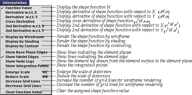
Setting the rendering mode
There are 3 different modes of rendering the shape function: wireframe, shading
and contouring. The mode can be set by choosing the corresponding item from
![]() menu.
menu.
|
“Display by Wireframe” : Choose this item to render the shape function in wireframe. The grid lines of the interpolation model are drawn with hidden line removal. |
|
| “Display by Shading” : Choose this item to render the shape function in shading. The interpolation model is rendered by smooth shading. | |
| “Display by Contour” : Choose this item to render the shape function by contour. The interpolation model is re p resented by contour line. This rendering option is useful especially for examining the inter- element continuity of the shape function derivatives. |
There appears check mark in front of the menu item set for the rendering mode.
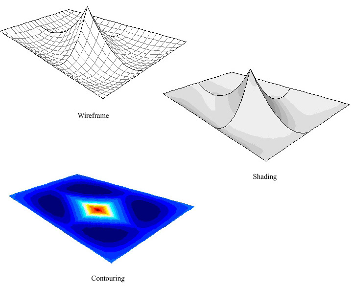
< Modes of rendering the interpolation mode >
Turning on or off supplementary lines in rendering
Supplementary lines may be added to therer rendered image of the interpolation model to improve its visual clarity. Choose the following items from menu to turn on or off the corresponding supplementary lines.
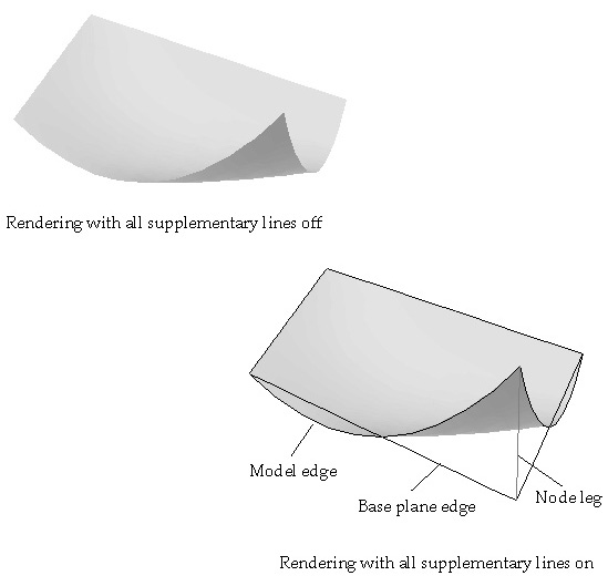
<Supplementary lines for the interpolation model >
Enlarging or reducing the value scale
The shape function or its derivative is expressed graphically as the height of the interpolation model over the base plane. The value scale implies the height re p resenting unit value of the shape function or its derivatives. If the scale is larger, the interpolation model is represented as a more steep surface.
The value scale can be adjusted. The scale is enlarged by choosing "Enlarge
Scale" item, and reduced by choosing “Reduce Scale” item
from ![]() menu.
menu.
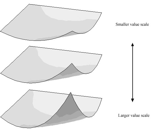
< Adjusting value scale >
Increasing or decreasing the grid lines of interpolation model
If the rendering mode is set as “Display by Wireframe,” the
interpolation model is represented by a number of grid lines. If necessary for
better visualization, the number of grid lines can be adjusted. The number of
grid lines increases, if “Increase Grid Lines” item is selected
from ![]() menu, and decreases, if “Decrease Grid Lines” item is selected.
menu, and decreases, if “Decrease Grid Lines” item is selected.
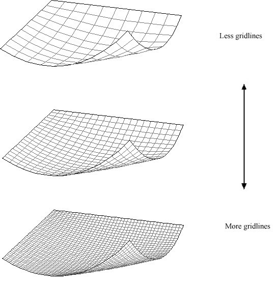
< Adjusting grid density >
Transforming the view of the interpolation model
For more detailed description on the use of the tool palette, refer to the "View Control" section in Chapter 2.
Scrolling, resizing and zooming the window
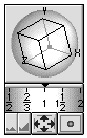
The contents of “Shape Function” window can be scrolled using horizontal or vertical scroll bars. The window may be resized or zoomed if necessary, by dragging the resize box or clicking the zoom box of the window.
|
|
|
|