Processing of structural analysis
The simplest method of getting a finite element solution is to use VisualFEA's
own processing capability. The finite element solver's capabilities are embedded
within VisualFEA. This makes VisualFEA much simpler to use than other finite
element p rograms which has separate module for processing, preprocessing and
postprocessing. In order to get into the processing stage for solution, choose
"Solve" item from  menu Then, "Analysis Options" dialog appears on the screen. The contents
of the dialog vary depending on the type of solution as will be described below.
Set the dialog items as desired and click
menu Then, "Analysis Options" dialog appears on the screen. The contents
of the dialog vary depending on the type of solution as will be described below.
Set the dialog items as desired and click  button.
Then, the processing starts, and goes on up to the completion of all the necessary
computation including assembling the system equations and solving them.
button.
Then, the processing starts, and goes on up to the completion of all the necessary
computation including assembling the system equations and solving them.
> Setting analysis options for linear static analysis
Choosing "Solve" item from
menu will pop up "Analysis Options" dialog as shown below, if you
have set the solution type as linear static.
The solution type is initially set as linear static, and remains as it is,
unless you have checked any one of the check boxes under "Solution Type",
i.e., "Material nonlinear", "Geometric nonlinear" and "Dynamic."
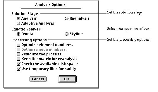
The dialog has a few items setting the options related to the finite element
solution procedure.
| |
solution stage: The solution stage may be set as one of "Analysis",
"Reanalysis" and "Adaptive." If
you turn on "Adaptive" radio button, the solution procedure
turns into adaptive process. The analysis options for adaptive analysis
are described in the next section. So, only "Analysis" and "Reanalysis"
options are described in this section. The initial default setting of
the solution stage is "Analysis" which leads to the normal procedure
of processing based on assembling equations and solving them. Once the
system equations are assembled and solved, they may be used for subsequent
processing by setting the option as "Reanalysis" The reanalysis
option will eliminate most of the computing time for assembling and decomposing
the system equations. The reanalysis option is enabled and valid only
under the following conditions.
|
| |
|
- The system equations should have been solved in the previous session.
|
| |
|
- The files containing the system equations should exist in the same
directory (folder) as the data file.
|
| |
|
- Geometry, element properties, and boundary conditions should not have
been altered since the system equation files were created.
|
| |
|
- The analysis type is linear static, and not adaptive nor sequential.
|
| |
equation solver: You may choose one of two
methods of assembling and solving equations: frontal method and skyline
method. They are typical and the most widely used methods in finite element
analysis solvers. Skyline method uses only CPU memory, while frontal method
relies much on auxiliary memory such as a hard disk. Accordingly skyline
method demands much larger CPU memory space than frontal method. Skyline
method usually works faster than the frontal method which requires frequent
reading and writing with the auxiliary memory. The default setting is "Frontal."
If your computer is equipped with huge CPU memory, and you want faster solution,
choose "Skyline." Otherwise, you should keep the option as "Frontal."
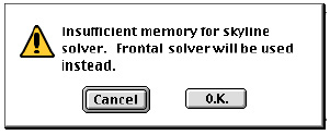
In case you chose "Skyline," but the memory space is not sufficient,
the software will notify this by the following message box. If you click
button
of the dialog, the software will automatically switch the solver to "Frontal." |
| |
|
| |
processing options: You can turn on or off each of the processing
options by clicking the check box in front of each item. These settings
are applied during the processing stage. |
| |
|
- "Optimize element number" : This item is
enabled only when the equation solver is set as "Frontal" If
this option is turned on, optimization of element numbering is automatically
done prior to assembling the system equations.
|
| |
|
- "Optimize node number" : This item is enabled
only when the equation solver is set as "Skyline" If this option
is turned on, optimization of node numbering is automatically done prior
to assembling the system equations.
|
| |
|
- "Visualize the process" : If this option is turned on, a
graphical rendering of the model is provided along with the status of
the element stiffness matrix assembly.
|
| |
|
- "Keep the matrix for reanalysis" : The system equation files
are created at the start of matrix assemblage and removed
at the end of the processing. In order to keep these files for reanalysis,
this option should be turned on.
|
| |
|
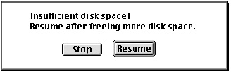
- "Check the available disk space" : If this option is turned
on, the available disk space is checked while processing is going on.
If the disk space is not sufficient, the processing will pause with the
following notice so that you may secure enough space and resume the processing.
|
| |
|
|
| |
|
- "Use temporary file for safety" : If the
processing is abnormally interrupted due to system failure or any other
reasons, the data file may be spoiled or lost. In order to avoid such
risks, turn on this option. Then, a duplicate of the data file will be
created temporarily and used during the processing, and it will replace
the original file when the processing is successfully completed. The processing
procedure is initiated when you click button
of the dialog, after setting all the appropriate items.
|
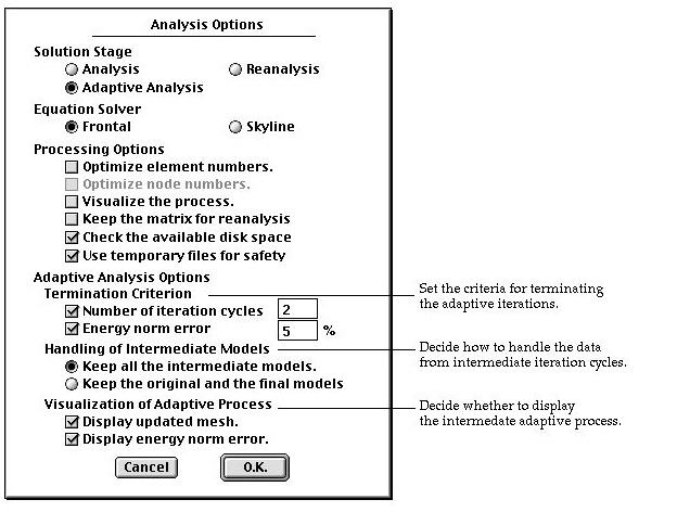
> Setting analysis options for adaptive analysis
If you click "Adaptive analysis" radio button of "Analysis Options"
dialog, the dialog expands with additional items as shown below. The upper part
of the dialog has the original items, and the bottom half includes new items
as follows:
| |
termination criterion: The adaptive iteration continues
until one of the conditions set for its termination is satisfied. These
conditions are termed here as the termination criterion. You may validate
or invalidate each one of the following termination criteria by checking
or unchecking the boxes in front of them. If the box is checked, the corresponding
criterion is applied.
|
| |
|
- number of iteration cycles: The number of iteration
cycles can be restricted by checking this item, and setting the number.
Iteration terminates when the number of cycles reaches the number.
|
| |
|
- energy norm error: Iteration terminates when maximum
energy norm error over the whole solution domain gets smaller than the
criterion set as the limiting energy norm error. If both of the termination
criteria are checked, iteration terminates when any one of them is fulfilled.
|
| |
|
 |
| |
handling of intermediate models: It is
the option determining how to treat the model data created at the intermediate
stages of iterations.
|
| |
|
- "Keep all the intermediate models": If this radio button
is turned on, the modeling data and analysis results obtained during the
intermediate cycles of adaptive iteration are saved, and can be retrieved
for later use.
|
| |
|
- "Keep the original and the final models": If this radio button
is turned on, the intermediate modeling and analysis data are discarded,
and only the original and the final data are saved.
|
| |
visualization of adaptive process: It is the option related
with visualizing the model and/or energy norm error while the adaptive
iteration process is going on.
|
| |
|
- "Display updated mesh": If this radio button is turned on,
the meshes generated at each step of adaptive iterations are plotted.
|
| |
|
- "Display energy norm error": If this radio button is turned
on, the energ y norm error distribution is displayed by contour at each
step of adaptive iterations. (This option may not work for the current
version of VisualFEA.)
|
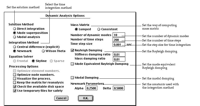
> Setting analysis options for dynamic analysis
Choosing "Solve" item from menu
will popup "Dynamic Analysis Options" dialog as shown below, if you
have set the solution type as dynamic. The solution type
can be set by using the "Project Setup" dialog.
| |
solution method : This option determines how to get
the dynamic analysis results. VisualFEA supports 3 methods of performing
dynamic analysis.
|
| |
|
- direct integration: No transformation is applied for integration in
time. The nodal displacements are obtained directly at each time step.ble
solution.
|
| |
|
- mode superposition: Time integration is operated on the participation
factors of dynamic modes. Thus, the dynamic modes are
extracted first through eigenvalue analysis, and the system equations
are formed in terms of participation factors of these dynamic modes. The
nodal displacements are obtained by superposing the dynamic modes at each
time step.
|
| |
|
- modal analysis: Only dynamic modes are extracted, No time integration
is performed. Other analysis results including nodal displacements are
not computed.
|
| |
integration method : This applies to the
integration in time for both the direct integration method and the mode
superposition method.
|
| |
|
- "Central difference (explicit)": A explicit
integration method, in which the stiffness matrix is not decomposed. The
mass matrix is decomposed only when consistent mass matrix is used. The
solution may diverge if the time step is larger than the critical value.
|
| |
|
- "Newmark": An implicit method with linear
acceleration controlled by parameters a and d, which can be set by the
user.
|
| |
|
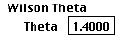
- "Wilson Theta": An implicit method with
linear acceleration controlled by an input parameter q, which can be set
by the user.
|
| |
mass matrix : There are following two options
in computing the element mass matrix.
|
| |
|
- "Lumped": The mass matrix is computed by assuming that element
mass is concentrated at nodal points.
|
| |
|
- "Consistent": The mass matrix is computed by interpolation
consistent with that used for the stiffness matrix.
|
| |
number of dynamic modes : To specify the number of dynamic
modes used for mode superposition. This item is valid only when the solution
method is set as mode superposition.
|
| |
number of time steps : The number of steps included for time
history analysis. The total duration of the analysis is determined by
the number of steps and the step size which is the next input item.
|
| |
time step size : The length of time from one step to the
next. Equal step size is assumed for the whole duration of the analysis.
|
| |
Rayleigh damping : If this item is checked,
Rayleigh damping is assumed,
|
| |
|
which is the form of 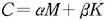 .
And the following 2 sub-items pop up. .
And the following 2 sub-items pop up.
|
| |
|
- "Stiffness damping ratio": This is the stiffness damping
coefficient b of the above equation.
|
| |
|
- "Mass damping ratio": This is the mass damping coefficient
a of the above equation.
|
| |
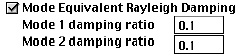
mode equivalent Rayleigh damping : If this item is checked,
Rayleigh damping is assumed, but is re p resented by 2 modal damping ratios
which appear as additional input items.
|
| |
|
- "Mode 1 damping ratio": 
|
| |
|
- "Mode 2 damping ratio": 
|
| |
|
|
| |
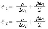
There is a following relationship between the Rayleigh
damping coefficients( and ) and the modal damping ratios (
and
). |
| |
|
|
| |
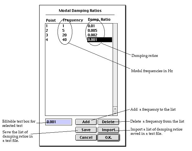
modal damping : One method of assigning damping characteristic
is to assume an individual damping ratio for each dynamic mode. It is
termed here as modal damping. However, information on dynamic modes is
not available prior to completing the modal analysis. Thus, the damping
ratio are specified as a function of modal frequency.
|
| |
If you click this item, there appears  button
which is used to launch "Modal Damping Ratio" dialog. A table
of modal frequencies and paired damping ratio can be specified using this
dialog. The damping ratio for a given frequency is estimated by interpolating
the values given in this table. button
which is used to launch "Modal Damping Ratio" dialog. A table
of modal frequencies and paired damping ratio can be specified using this
dialog. The damping ratio for a given frequency is estimated by interpolating
the values given in this table.
|
| |
 |
| |
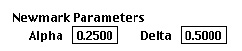
Acceleration parameters : parameter(s) for
linear acceleration of time integration. There are different parameters
depending on the method of time integration. The input items change as
the method of integration changes.
|
| |
|
- central difference method: no input parameters for
this method of integration.
|
| |
|
- Newmark: There are 2 parameters a and d. The default values, a=0.25
and d=0.5 are used for unconditionally stable solution.
|
| |
|
|
| |
|
- Wilson ąŔ: There is a parameter q. The default value is q=1.4. The value
of should be 1.37 or greater for unconditionally stable solution.
|
> Setting analysis options for nonlinear analysis
Choosing "Solve" item from
menu will pop up "Nonlinear Analysis Options" dialog as shown below,
if you have set the solution type as material nonlinear, or geometric
nonlinear. The solution type can be set by using the "Project Setup"
dialog.

| |
number of load incremental steps : It is the number
of steps for solution of a nonlinear problem by incremental
method. If this value is 1, a simple iterative solution is applied. Otherwise,
the total load is divided into as many segments as this number, and applied
incrementally through the nonlinear solution process.
|
| |
number of iterations within a step : The maximum limit in
the number of iterations within an incremental step for solution of nonlinear
equation. If this value is 1, simple incremental procedure is applied.
|
| |
error tolerance for convergence
: This convergence criterion applies to the iterative
procedure within an incremental step. The iteration is terminated if either
the percentage of the residual force falls below this level, or the number
of iterations reaches the maximum limit.
|
| |
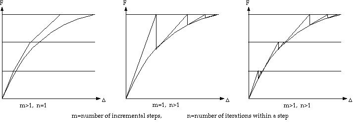
< Number of load increments and number of iterations
>
|
| |
options for stiffness matrix update: There are following
3 options of updating stiffness matrix throughout the incremental and
iterative process.
|
| |
|
- "Constant stiffness matrix (no update)": If this button is
turned on, the stiffness matrix is not updated throughout the whole incremental
and iterative process. Thus, the stiffness matrix is computed only once
and no additional time is required for its update. However, this option
leads to large number of iterations as shown in the figure below.
|
| |
|
- "Update each step of load increment": If
this button is turned on, the stiffness matrix is updated only for the
first iteration of each load increment. The stiffness matrix remains constant
for all iterations within a load incremental step.
|
| |
|
- "Update each iteration within a step": If this button is
turned on, the stiffness matrix is updated for every iteration throughout
the whole process. This option takes more time for updating stiffness
matrix, but requires smaller number of iterations.
|
| |
|
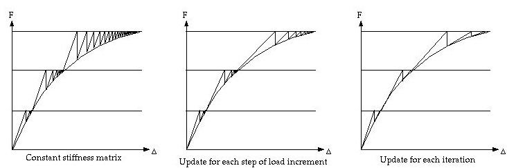
< Schemes of stiffness matrix update >
|
| |
other nonlinear option:
|
| |
|
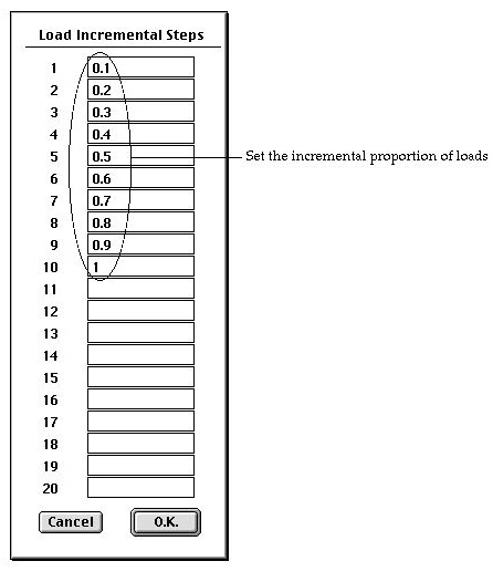
- "Specify division of incremental
steps" : This item is not checked by default, and the sizes of all
load increments are equal. If you check this item, the following "Load
Incremental Steps" dialog pops up. Initially the editable text boxes
are filled with uniformly divided incremental portions of the load. These
incremental proportions can be modified by editing the text. boxes |
| |
|
 |
| |
|
- "Keep results of intermediate steps" : If this
item is checked, the solution data obtained at every incremental step is
saved, and can be retrieved for later use. |
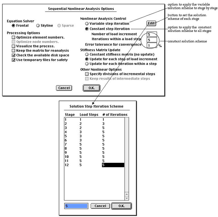
> Setting analysis options for sequentially staged modeling
As for linear analysis, the same dialog is used for both non-staged and staged
modeling. In the case of nonlinear analysis, dialog for sequentially staged
modeling has a few more items than the dialog for non-stage modeling. They are
related to incremental and iterative solution scheme for each stage. In order
to apply constant number of incremental steps and iterations, turn on "Constant
step iteration" radio button in the dialog and then insert the number of
incremental steps and iterations in the editable text box. In order to differentiate
the incremental and iterative scheme from stage to stage, turn on "Variable
step iteration" ratio button. And click  button.
Then, "Solution Step Iteration Scheme" dialog appears. You may set
the number of load steps and the number of iterations using this dialog. The
dialog displays as many rows as the number of stages. At the beginning , each
row is assigned with equal number of incremental steps and equal number of iterations.
Set new values by editing the existing ones, and click button
to complete the setting.
button.
Then, "Solution Step Iteration Scheme" dialog appears. You may set
the number of load steps and the number of iterations using this dialog. The
dialog displays as many rows as the number of stages. At the beginning , each
row is assigned with equal number of incremental steps and equal number of iterations.
Set new values by editing the existing ones, and click button
to complete the setting.